
The Final "Ilya's Papers to Carmack" Paper: Neural Scaling Laws
So long and thanks for all the fish

This post is part of a series of paper reviews, covering the ~30 papers Ilya Sutskever sent to John Carmack to learn about AI. To see the rest of the reviews, go here.
This is the last paper review in my “Ilya’s papers” series. I’ve been working on this series on and off for over a year, and it’s weird to say that it’s finally done. Of course, I’ll keep reviewing papers in general. I have a long backlog of more modern papers that I would love to write about. But I’m never going to write another paper in the Ilya’s papers series, and that alone is strange. I started this series when I had 38 subscribers, and now there are ~35x that in this little corner of the web. Thank you all for coming out to read my ramblings. I’d say that I couldn’t have done it without you, but that’s not really true because all the content was free and I would’ve written whether or not you were there.

Paper 23: Scaling Laws for Neural Language Models
High Level
Imagine you’re running a restaurant. You’re trying to sell burgers, and you want to make money doing it. You have the basics — you got your restaurant and you have your patties and buns and you got a square yellow fry cook in the back. After your first month you made $1000 that you can put back into the restaurant. Good job! Now how do you spend it to make the most money possible the second month?
There are a lot of options. A lot of them are probably dumb. You probably won’t make more money if you spend those $1000 handing out flyers to vegans, for example. But there are a lot of options that are not dumb. You could buy more patties and buns. You could hire another fry cook. You could spend money on Facebook to target burger lovers in your area. How do you make that money go as far as possible?
We’ve built up a ton of rules and knowledge and heuristics about how to answer that question. Arguably, the MBA is entirely about learning how to answer this question.
Ok, same question, but now with neural networks. You have $1000. How do you spend it? Should you buy more compute? Or more data? Should you increase your model parameter count? Or try and figure out if you can change the shape to get better cost efficiency? A few years ago, the answer to all of these questions was basically a big fat 🤷♂️ Practitioners had their theories with made up ratios1 but nothing concrete.
But in the late 2010s, a few related things happened. First, in the background, there was a debate raging about “the scaling hypothesis”. Do models get better as they get bigger? Does that improvement plateau? Or is scaling enough to take us to AGI/ASI? Ilya Sutskever, chief scientist at OpenAI, was a leading voice in the pro scaling hypothesis camp. And second, training large LLMs became critically important to OpenAI’s research direction, and as they got bigger they became more costly to train, and as they became more costly to train, the scrutiny over AI training line items increased in tandem. So you have this perfect mix of ingredients — the guy who believes in the scaling hypothesis is running a lab that is pushing the scaling hypothesis to the limits, and given limited resources the most important question for the lab is “how do we spend the incremental dollar to get the best model performance?”
Scaling Laws is an attempt to rigorously answer that question.
The authors begin by defining the option space. They only care about transformers. They only care about language learning using the standard auto regressive next token prediction task, in particular on the WebText2 dataset. They use test loss as their measure of improvement. And they define a set of variables that they want to empirically evaluate:
Model depth
Model width
Model architecture
Batch size
Training steps
Number of data samples
The approach is straightforward: train a ton of models with different values for all of these variables, and then plot the results and see if anything with predictive power comes out.
I think it’s worth just copying the final discoveries verbatim. But first, here’s the money shot:
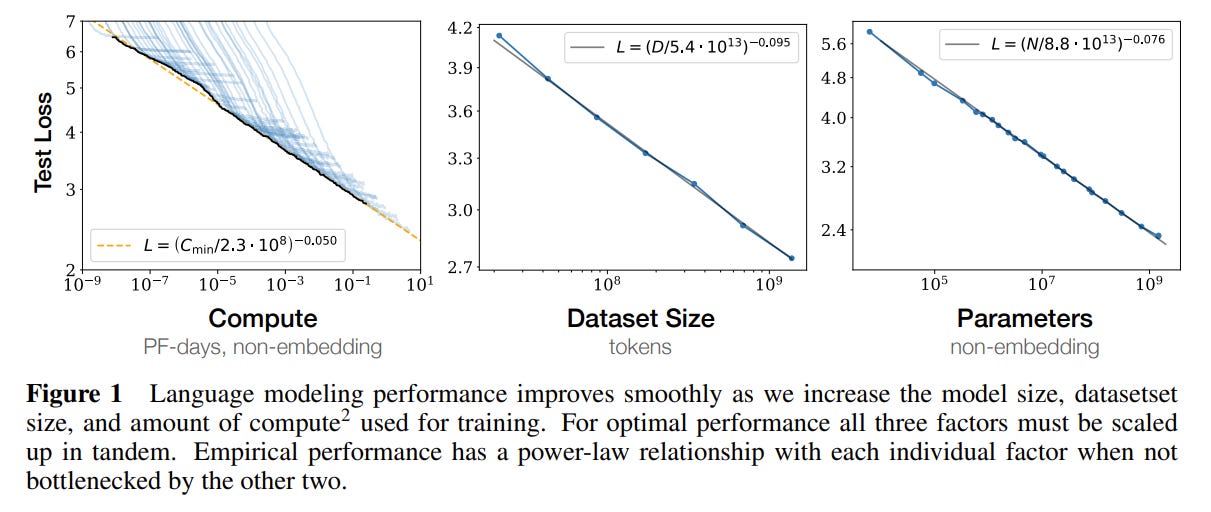
This figure is basically the entire paper. Empirically, it seems that neural network performance is a power law function of compute steps, dataset size, and model size over ~10ish orders of magnitude. If you only have one takeaway, it should be that graph.
Onto the actual results. From the paper:
Performance depends strongly on scale, weakly on model shape: Model performance depends most strongly on scale, which consists of three factors: the number of model parameters N (excluding embeddings), the size of the dataset D, and the amount of compute C used for training. Within reasonable limits, performance depends very weakly on other architectural hyperparameters such as depth vs. width.
Smooth power laws: Performance has a power-law relationship with each of the three scale factors N, D, C when not bottlenecked by the other two, with trends spanning more than six orders of magnitude (see Figure 1). We observe no signs of deviation from these trends on the upper end, though performance must flatten out eventually before reaching zero loss.
Universality of overfitting: Performance improves predictably as long as we scale up N and D in tandem, but enters a regime of diminishing returns if either N or D is held fixed while the other increases. The performance penalty depends predictably on the ratio N0.74/D, meaning that every time we increase the model size 8x, we only need to increase the data by roughly 5x to avoid a penalty.
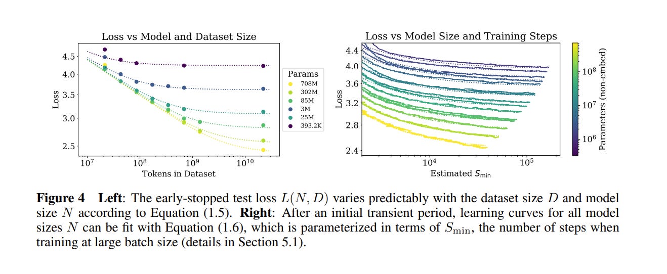
Universality of training: Training curves follow predictable power-laws whose parameters are roughly independent of the model size. By extrapolating the early part of a training curve, we can roughly predict the loss that would be achieved if we trained for much longer.
Transfer improves with test performance: When we evaluate models on text with a different distribution than they were trained on, the results are strongly correlated to those on the training validation set with a roughly constant offset in the loss – in other words, transfer to a different distribution incurs a constant penalty but otherwise improves roughly in line with performance on the training set.
Sample efficiency: Large models are more sample-efficient than small models, reaching the same level of performance with fewer optimization steps and using fewer data points.
Convergence is inefficient: When working within a fixed compute budget C but without any other restrictions on the model size N or available data D, we attain optimal performance by training very large models and stopping significantly short of convergence. Maximally compute-efficient training would therefore be far more sample efficient than one might expect based on training small models to convergence, with data requirements growing very slowly as D ∼ C0.27 with training compute.
Optimal batch size: The ideal batch size for training these models is roughly a power of the loss only, and continues to be determinable by measuring the gradient noise scale; it is roughly 1-2 million tokens at convergence for the largest models we can train.
For simplicity, I’m going to group our analysis of these experiments into four sections. These sections mostly follow the ordering of the paper, but I jump around a bit and combine experiments in a few places. Also, a quick note: the basic structure of this paper is ‘run a bunch of experiments to gather observations, and then fit a line to the trends’. This seems like a complicated paper with a lot going on, but if you understand that core mechanism of insight generation the rest of this should be easy to understand.
Understanding model shape
The first set of experiments examines how model shape at fixed parameter count impacts performance. The most obvious knobs to turn are the ones that come “out of the box” with transformers: how many layers (depth), how many parameters per layer (width), how many attention heads. And it may also be worth looking at the ratio of these terms. Maybe there’s a magic depth to width ratio where things work great. If you can only support a model with N parameters — say, due to memory limitations — is it better to use those parameters to increase model width, or depth, or something else?
Surprisingly, it seems that it doesn’t really matter how you allocate your parameters. Take a look at these graphs:
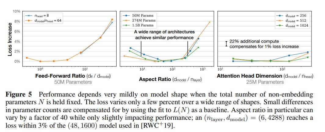
In each case, the authors change the ratios of various model hyper parameters a lot. To pick a specific example, they change the ratio of the model residual stream and the number of layers from 1 to 1000. And the delta in the performance (as measured by the test loss) is, at most, only a few percent. This is really weird! Here are two different model shapes:
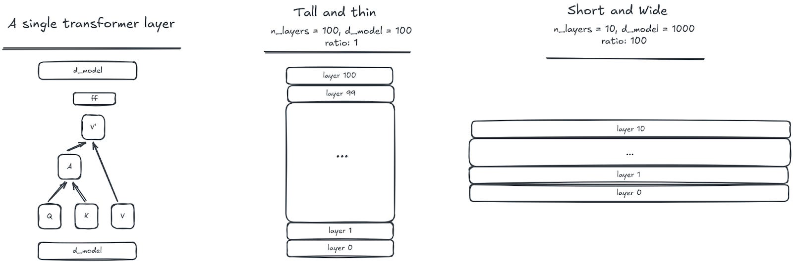
You’re telling me these have the ~same performance?! Conventional wisdom is that depth and width matter a lot!
Part of why this flies in the face of intuition is that we often use increases in layers and width without strictly controlling model parameter count. When there is some model performance gain, it is easy to attribute some amount of the gain to the parameter increase, and some to whatever specific intervention you made. I suppose someone had to be the first person to actually test that hypothesis rigorously!2
What’s especially interesting is that shape seems to not really matter for a wide range of model sizes. The number of parameters seems to be the primary driver for how well a model does; any particular configuration is only going to move the needle a few percent at most. For anyone who has ever done painful hyperparameter grid searches, this is perhaps a breath of fresh air. You do not really have to worry about whether your particular research innovation is being sabotaged by bad hyperparameters; and there is less reason to feel compelled to do just one more iteration of tuning to try and get better results. But assuming these results hold for architecture outside of transformers, it also means that vast amounts of literature related to micro-optimizations are probably not worth the paper they were printed on.
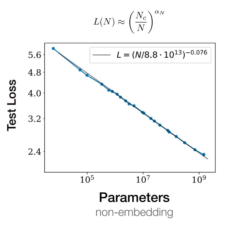
The authors use all of this data to derive their first scaling law: the relationship between loss and parameter count.
Speaking of other architectures. If you expand the aperture of ‘shape’ a bit, you may also want to ask whether decoder-only transformers are really the best thing since sliced bread. LSTMs are also very powerful (cf link); maybe lstms are actually as good as transformers?
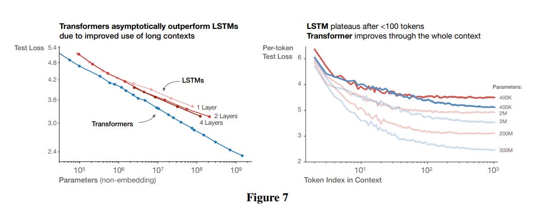
Here our intuition serves us better. Transformers seem to linearly improve with size while LSTMs eventually taper off, in large part due to their difficulty in handling longer sequences. Note that this is accounting for parameter size, so we can’t just round it off as transformers having more compute per token. There is something about transformers that make them pound for pound better than LSTMs.
Understanding compute / data relationships
The second set of experiments aims to establish compute/data scaling laws. These experiments are detailed entirely in a few paragraphs in section 3.3. But don’t be fooled by the lack of ink — this is probably the most important part of the paper.
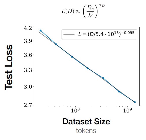
The authors first detail their dataset size experiments. They slice the WebText2 dataset into a bunch of slices, and create 7 subsets of increasing size to simulate different amounts of available training samples. The smallest dataset is ~107 tokens; the largest is ~109. The authors fix everything else — available compute, model size, batch size, model shape, etc — and then train models and evaluate the lowest test loss each model achieved. The resulting trend line is straightforwardly predicted by a power law, giving us the second scaling law.
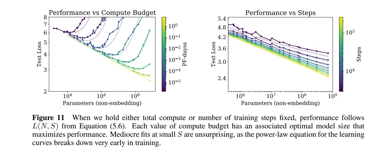
Next, the authors dig into compute, measured in total flops. Note that compute is not the same thing as model size. For a certain flop budget, you can have one really big model that you run for a small number of steps, or a small model that you run for a lot of steps. In order to accurately measure how compute relates to performance, we need to vary both total compute and find the optimal model size for each compute amount.
The authors estimate total flops as C = 6*N*B*S, where N is the number of parameters, B is the batch size per step, S is the number of steps, and 6 is to account for forward and backwards updates per parameter. If you rearrange slightly3, you get:
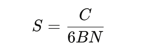
You can think of this as “the step where a model of size N has used exactly C compute.” From here, the authors train a bunch of models of different sizes i.e. at a bunch of values of N. They calculate the loss of each model at each step. They calculate the amount of compute each model has used at that step.4 And then they simply find the model with the lowest loss for each value of compute. That gives us the third scaling law:
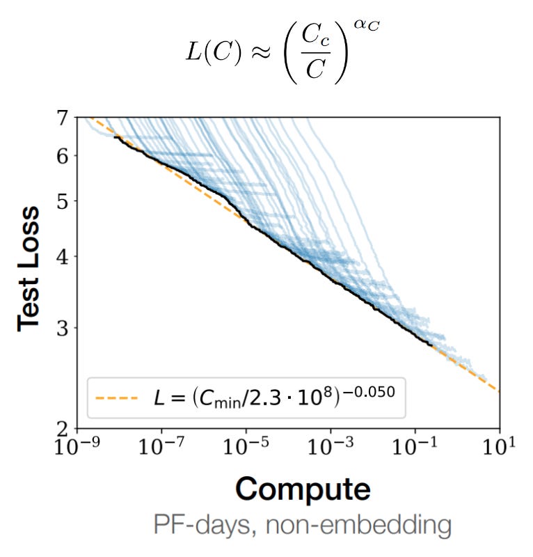
What can we gather from all this? The first scaling law says that larger models result in better performance. The second scaling law says that more data predictably results in better performance. And the third scaling law says that more compute — either through larger models or through more training steps — results in better performance.
In some sense, this is obvious, and matches everyone’s intuition.
But now we can predictably say how much we expect each axis to matter. First, none of these improve linearly. They are all following power laws, which means there are diminishing returns. You need to get x more compute to go from a to b, but then you need y more compute to go from b to c. Second, given a certain configuration of variables, we can approximately predict what the final performance will be before we start a single training run. In a world where each training run costs millions of dollars, this is a huge benefit. Finally, we can estimate exactly how long we should push each training run. In particular, we have some hard evidence that it does not make sense to train models all the way to convergence. More on this in the later sections.
Ok this is all well and good, but we are basically never considering any of these questions in isolation. If I have $100, I could spend it on data, or on a bigger model, or both! Can we define a useful equation that will help us predict what the loss may be as a function of both the number of data points and the size of the model?
The authors work backwards.
They know that if you fix the total amount of data and make the model infinitely large, the loss should approach the data scaling law above. And by the same token, they know that if you fix the model size and make the amount of data infinitely large, the loss should approach the model scaling law above. (In other words, your loss is capped by where you are most resource constrained).
They know that changing the vocabulary size or the amount of tokens should ‘rescale’ the loss. Transformers use a cross entropy loss that calculates the sum of the errors across all of the tokens in a vocabulary. If you wanted to calculate a per-token loss, you would average that sum over the total number of tokens. Switching from word-level tokens to character-level tokens would massively decrease the total quantity of tokens available, but the model may not actually be any worse at prediction. The choice of how you tokenize text is a convention, and the authors want to create a scaling law that describes something physically meaningful about learning that’s invariant to conventions. This is like requiring that physical laws are invariant to which units you choose to use.
They hypothesize that the loss is “analytic” as the amount of data increases — that the loss function is essentially a smooth, boring function with derivatives everywhere and no weird jumps or cuts or anything like that as the data gets really large. This is somewhat intuitive. We would not expect that adding a single new (independent) data point will magically result in really big changes to the loss outcome.5
The authors propose this loss function:
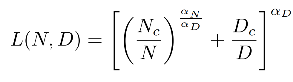
as the optimal loss for a model of size N trained on D data points.
To test their hypothesis, the authors do the same thing they did before: train a bunch of models, see the loss, and see how well their equations fit the empirical data.
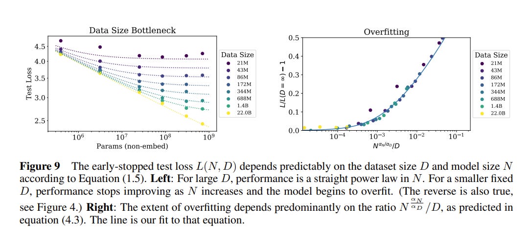
The strongest justification for their equation is that it seems to map pretty well to the data. Note especially that the larger the dataset size, the more accurate the loss prediction. With this equation in hand, we can be pretty confident about what the optimal test loss will be for a given model before we’ve done any training at all.6
Understanding model size / training time relationships
Up until now we’ve spoken about how data and model size relate to each other under optimal training conditions. But what does that last part mean? What is an ‘optimal training condition’? Well, mostly it relates to how you spend the compute you have in front of you.
Earlier I said:
For a certain flop budget, you can have one really big model that you run for a small number of steps, or a small model that you run for a lot of steps. In order to accurately measure how compute relates to performance, we need to vary both total compute and find the optimal model size for each compute amount.
In this section, the authors try to figure out that trade off.
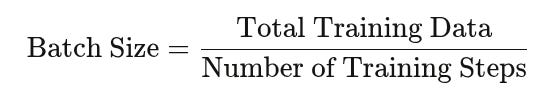
First, some basics. As we saw above, if you assume that your model size is constant, your test loss is based on the number of data points that you train on. So, in order to understand how long you should train a model, you need to tie together the number of training steps with the number of data points. You do that with batch size, which naively is just:
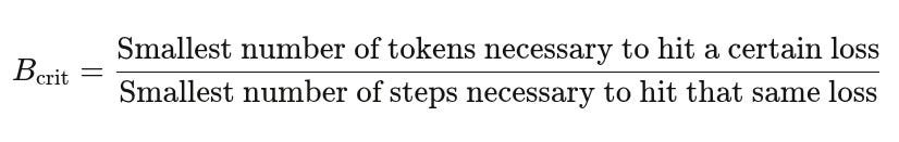
To achieve some target loss as quickly as possible, there is an ‘optimal batch size’. The conventional wisdom is that you want to have the largest batch size possible, because that makes your gradients more stable and results in more accurate model updates. But large batch sizes mean fewer training steps over a fixed compute budget. To use training time and compute as effectively as possible, we want to set our batch size to a specific ‘critical batch’ value. Anything more would minimize training steps at the expense of compute; anything less would minimize compute at the expense of training time. Tautologically, you can define the critical batch size as:
How do you find the exact batch size where you hit diminishing returns? This is a very empirics driven paper, so of course the authors simply train a bunch of models to find the optimal batch size for various losses.
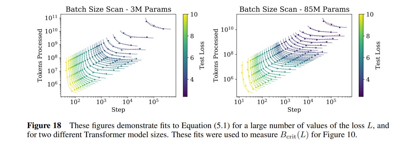
Two interesting takeaways:
Empirically, the critical batch size is not related to the size of the neural network being trained! This is surprising — intuitively you would expect that a larger model would have more ‘capacity’ to handle more data points at a time. But in fact, that is not the case: gradients apply to the entire model, so large and small models are impacted equally by batch size.
The optimal batch size increases as the model gets better during training! If you train with a static batch size over the course of an entire training run, you are potentially leaving a lot of efficiency on the table. This may be because, as time goes on and the model performance improves, the cost of noisy gradients becomes an outsized issue.
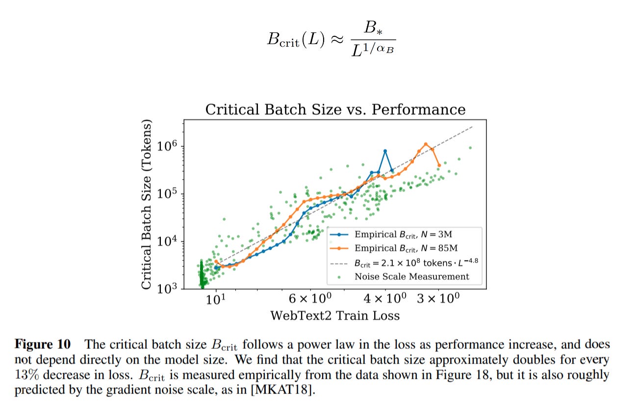
The authors take the data from above and plot it against the loss achieved and fit a power law as a function of loss.7 8
Earlier, the authors defined a bunch of relationships between data size and compute size, but did not take batch size into account. Their earlier experiments were done with a fixed batch size, B = 219 tokens. That means their experiments were all inefficient in some way. Can we use that data to figure out what the minimum number of steps would be? Yes — the authors find the relationship between the optimal number of steps at Bcrit and the observed number of steps at B as:
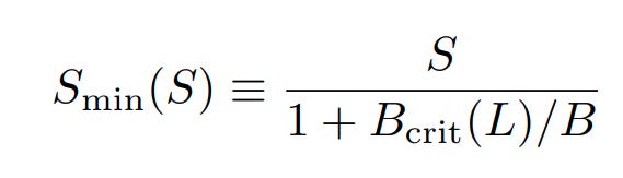
Where Smin is the smallest number of steps to achieve target loss L at batch size Bcrit, given observed number of steps S at batch size B.
We said that a given amount of compute could be spent on a larger model or on more training steps. Given infinite data, how should you apportion out your compute budget? With the above math, we can come up with an answer.
With infinite training data and infinite training time, loss scales as a power law dependent on model size. And with a sufficiently large model and infinite data, loss scales as a power law dependent on training steps. The authors propose that you can additively combine these to get a loss equation that is dependent on both model size and training time:
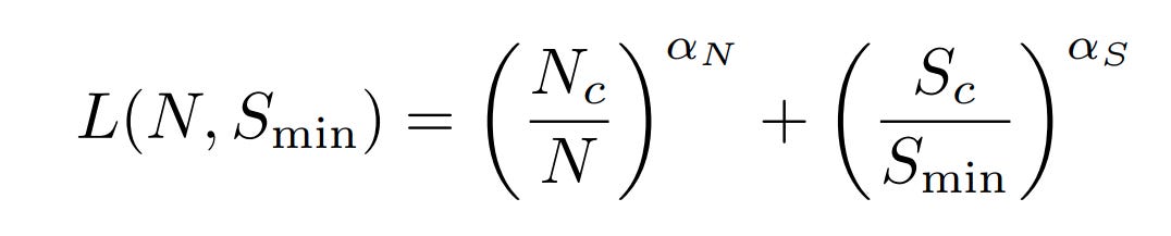
And, of course, back this up by fitting a bunch of data points to the generated curves.
These results also let you estimate approximately when you should stop training your models (early stopping). I’ll leave this bit out of the review, but check out section 5.3 if you are curious.
Optimality and contradictions
We have everything we need now to figure out how to apportion out a given amount of training compute between model parameters, batch size, and training steps. The result:
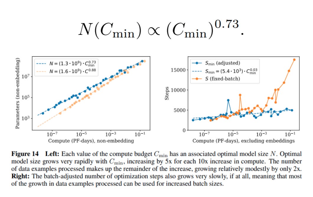
In other words, the vast majority of compute should go to model size. Most of the rest goes to larger batch sizes. And the number of training steps barely increases.
So, with all of the above, we have something that looks a bit like a mechanistic framework for understanding LLMs. To quote the authors:
Our scaling laws provide a predictive framework for the performance of language modeling.
There is one interesting hiccup in the paper: even though these scaling laws seem to hold for many orders of magnitude, there is a built in contradiction. From the experiments above, we know how loss relates to data; and how loss relates to compute; and how compute relates to data. If we represent the data curve in terms of compute, and follow the trend lines, we get:
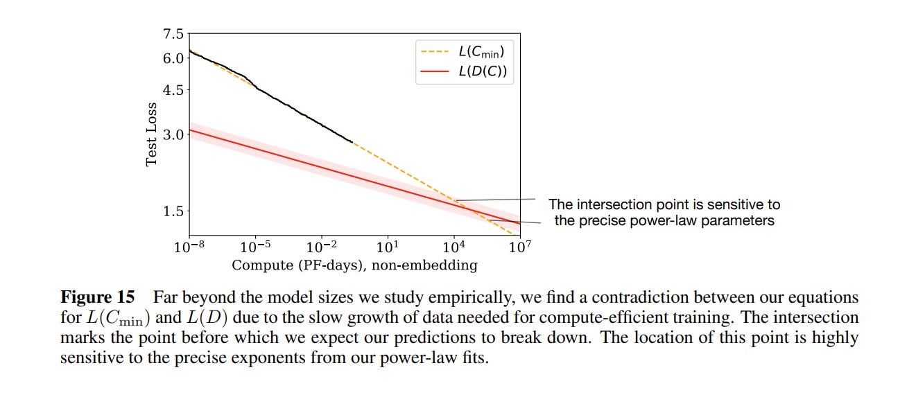
At 104 petaflop days of compute, the performance predicted by the compute trend line drops below the bound defined by the data trend line. So somewhere before 104 peta-flop days of compute, these scaling laws have to break down.
Where does the contradiction arise? The red line in the graph above is the L(D) bound — the predicted loss given a certain amount of data. It comes from empirical analysis for when models start to overfit, and empirically seems to follow this equation:
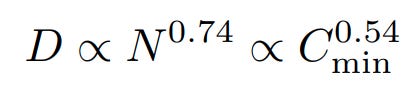
If you rewrite the equation for compute efficient training with the optimal critical batch size and assume you never do more than one epoch of training, you get:
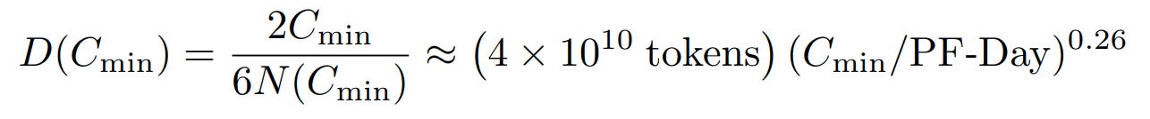
Which grows way more slowly. In other words, “compute-efficient training will eventually run into a problem with overfitting, even if the training process never re-uses any data!” Either the L(D) is wrong, or something else breaks before we get to the intersection point.
Where is the intersection point? Well it’s very dependent on the constants you get from the line fits. But the authors calculate it as:

For context, GPT3 was released in 2020, around when this paper was written. It had about 1011 parameters. The authors go so far as to speculate that this intersection point may represent the max representational capacity of transformers. (Actually, they just got L(D) wrong. See below.)
Insights
First, a few thoughts on the actual meat of the paper, things that stood out and things that helped me reason through my own mental models for how deep learning works.
I was very surprised to read that it is never optimal to train a model to convergence. In retrospect this makes some sense. Every model training curve has a clear inflection point between a steep part, where the model learns things quickly, and a flat where there are diminishing returns. So of course, you should always try to keep your model training in the steep part where possible, taking advantage of your compute to train larger models! There are two complications.
Practicality. It wasn’t always easy to leverage compute in really flexible ways. In 2026 you can sorta kinda abstract over large clusters of GPUs to train arbitrarily large models. In 2018? Your model better fit on that one GPU!
Complexity. The convergence analysis doesn’t account for ‘grokking’, an observed behavior where a neural network will suddenly see a sizeable drop in loss. This seems to come from ‘phase transition’-like behavior within neural network internals (cf the monosemanticity paper from Anthropic). Perhaps the analogy is apt. The Scaling Laws paper was inspired by ‘ideal gas laws’ in physics. The gas laws are also more or less accurate, except for areas where there are phase transitions from gas to liquid / solid.
Similar thought on batch size. I was taught that larger batch sizes == better, and minibatching is essentially a compromise due to limited compute resources. Back then, gradient stability was such a big problem that nobody would imagine purposely using noisier gradients for speed. But we more or less solved the stability thing with better optimizers and better architectures, and now compute is the biggest bottleneck, so trading off stability for compute efficiency is a good trade.
I was also surprised to find that larger models are significantly more sample efficient — a big model can reach the same loss as a small model with fewer steps. To try and guess at why, I think mechanically there are ‘more’ gradient updates in a larger model because there are more parameters, so the model is able to extract more per data point. The additional parameters learn ‘nuance’ much more quickly. But this is really just a guess, and also flies in the face of my intuition for why critical batch size is model size agnostic. You could easily construct a just-so story for why smaller models would be more efficient, and I would likely believe that too.
Not all of these scaling laws are accurate. Because these laws were derived primarily from empirics, any bias in the experimental design could result in different outcomes. One such bias: not varying the training schedule (learning rate decay) for runs of different lengths. The authors of Scaling Laws used the same learning rate schedule for all of their training runs, whether short or long. This had the effect of making shorter runs seem much worse, since they never had the ability to properly decay their learning rate. Scaling Laws argues that scaling compute is much more important than scaling the number of training samples, and as a result we spent three years with everyone trying to hoard as many GPUs as possible. Eventually, the folks over at Deepmind published Training Compute Optimal LLMs (AKA the Chinchilla paper), which argues that compute and data are roughly equally important. This also neatly resolves the contradiction mentioned above.
While we are talking about other papers, Scaling Laws has inspired an entire cottage industry of other scaling law papers. As I wrote in Towards a Language for Optimization:
[The scaling laws approach] worked great. In fact, it worked so well, it created a new kind of paper: the ‘scaling law’ paper, where researchers attempt to discover similar behaviors in a wide range of tasks and architectures. It turns out the findings replicate. The relationship between performance, compute, data, and model size is some kind of universal behavior — a power law modulo a constant. All of the complexity of neural nets, boiled down into 5 floats.
So where does that all leave us?
One of the reasons I really like this paper is because, with hindsight, it reads like a manual for the entire tech industry from 2020 to 2025. In this single paper you can see:
The sprint for more compute and the rise of NVIDIA
The sprint for more data, the exhaustion of text as a viable data source, and the rise of data providers
The need to search beyond standard pre-training scaling to continue driving improvements in models
And more.
There were several papers in Ilya’s list of ~30 that left me scratching my head. Why that paper? Of all of the papers out there, that one? This paper is not like that. Scaling Laws is perhaps the most consequential paper to come out of the tech industry since Map Reduce. Yes, even more so than the transformers work that it is built on. I often say that the AI world is built on intuitions instead of models, that no one really knows how to deal with these things. Scaling Laws decides to try anyway. Quoting again from Towards a Language for Optimization:
I can’t stress enough how useful this systems level understanding is. It directly informs macro strategy. Why was everyone trying to get compute in 2023/2024? Because the scaling laws said they were bottlenecked by compute. Why is everyone trying to get data in 2025 and likely into 2026? Because the scaling laws say they are bottlenecked by data. Every lab is trying to get the best model performance possible. And it turns out there’s a neat equation that directly maps <things you can change> to model performance. Of course the scaling laws will influence macro strategy!
I think that this paper fundamentally changed the practice of ML. The publication of this paper shifted us from ML Research to ML Engineering. How do you set your hyperparameters? How long should you train? How big should your batch size be? How many parameters? How much data? In 2019, all of this was vibes. Trust me, when I was training models at Google, it was a lot of vibes. Now, we can predict. Before we even start a training run, we can figure out roughly how well the model will perform.
And, as a result, pretraining is no longer all that interesting! We’ve figured it out! All the interesting work has shifted to post training regimes — reinforcement learning, human feedback, instruction tuning, prompt engineering — or to completely different domains, like world models or test time training (I promise I’ll review the Titans and Hope papers soon). When I talk to folks about pretraining, it’s all “how do I engineer my massively complex data center” and less “lets sit at a whiteboard and think about how models might behave.” Completely different personality type.
One last thought. It’s funny how, even though we’re ending this series, the conversation isn’t anywhere close to finished. In this final review, we are already linking to and talking about more recent papers. It’s all just one huge conversation, each new set of authors picking up where previous ones left off. In other words, more to say, more to be written. Thanks for joining me on this ride, and stay tuned for more paper reviews. I have notes for papers on diffusion modeling, speculative decoding, mechanistic interpretability, test time training, etc. and now that I’m done dragging my feet here we can get into some of the things that may be more immediately applicable for a modern ML researcher.
improvingI was often asked for advice by other Google teams about how to think about deep neural networks, and I’d often say that a dollar spent on better data was worth $100 spent on more compute
For depth specifically, the authors hypothesize that the residual stream makes transformers act as ensembles instead of as sequential layers. When a model has many layers stacked without residuals, each additional layer explodes the space of possible operations. When a model has layers stacked with residuals, each additional layer ends up learning a different modification on top of the residual stream, and there are simply not that many operations that will be meaningful. Eventually you hit diminishing returns. See the review of the ResNet paper.
Note: there is a typo in the paper.
Measured as petaflops/s * days, or PF-days.
Note that this is not true of model size! We totally expect that there are discontinuities between large models and small models, cf ‘grokking’.
Sort of. There are a few additional things that were not perfectly optimized, like dropout rate and batch size. We’ll get to those later in the post.
Note that this equation will diverge from the ‘true’ loss as the loss approaches 0. Because it is impossible to actually achieve 0 loss, this assumption seems reasonable.
The authors measure ‘gradient noise scale’ on the same plot. This is a number that measures the amount of ‘noise’ in your minibatch gradient update. Remember that the ‘true’ gradient is calculated over the entire dataset. Since we are using minibatches, we are only approximating the true gradient. The gradient noise scale measures the difference. When the batch size is small, we get more gradient noise. As you increase batch size, you decrease gradient noise. This happens linearly until the critical batch size, after which you get diminishing returns. The authors plot gradient noise scale next to the critical batch size to show that they are linearly reducing gradient noise throughout.